Nicolás Pavón
PREDICTING CHRONIC KIDNEY DISEASE
The issue:
Across the globe, many people are dealing with kidney diseases. These can show up suddenly due to various risk factors like what they eat, their surroundings, and how they live. Checking for these diseases can be invasive, expensive, and slow. It might even be risky. This is why, especially in places with limited resources, lots of patients don't get diagnosed and treated until their kidney disease is already advanced. So, finding ways to spot these diseases early is really important, especially in developing countries where late diagnosis is common.
The data:
There are many datasets containing information of patients with this desease that can be worked on to achieve our objective, predict chronic kidney disease. In this case we are going to use the dataset provided by the UCI repository. Looking at the description of the dataset and the data itself we can define the types and roles of the attributes:
Dataset info:
| Name | Abbreviation | UCI Description | Observed type |
|---|---|---|---|
| Age | age | Numerical | Integer |
| Blood Pressure | bp | Numerical | Real (in mm/Hg) |
| Specific Gravity | sg | Nominal | Polynomial (1.005, 1.010, 1.015, 1.020, 1.025) |
| Albumin | al | Nominal | Polynomial (0, 1, 2, 3, 4, 5) |
| Sugar | su | Nominal | Polynomial (0, 1, 2, 3, 4, 5) |
| Red Blood Cells | rbc | Nominal | Binary (normal, abnormal) |
| Pus Cell | pc | Nominal | Binary (normal, abnormal) |
| Pus Cell Clumps | pcc | Nominal | Binary (present, notpresent) |
| Bacteria | ba | Nominal | Binary (present, notpresent) |
| Blood Glucose Random | bgr | Numerical | Real (bgr in mgs/dl) |
| Blood Urea | bu | Numerical | Real (bu in mgs/dl) |
| Serum Creatinine | sc | Numerical | Real (sc in mgs/dl) |
| Sodium | sod | Numerical | Real (sod in mEq/L) |
| Potassium | pot | Numerical | Real (pot in mEq/L) |
| Hemoglobin | hemo | Numerical | Real (hemo in gms) |
| Packed Cell Volume | pcv | Numerical | Real |
| White Blood Cell Count | wc | Numerical | Real (wc in cells/cumm) |
| Red Blood Cell Count | rc | Numerical | Real (rc in millions/cmm) |
| Hypertension | htn | Nominal | Binary (yes, no) |
| Diabetes Mellitus | dm | Nominal | Binary (yes, no) |
| Coronary Artery Disease | cad | Nominal | Binary (yes, no) |
| Appetite | appet | Nominal | Binary (good, poor) |
| Pedal Edema | pe | Nominal | Binary (yes, no) |
| Anemia | ane | Nominal | Binary (yes, no) |
| Class | class | Nominal | Binary, and label (ckd, notckd) |
Importing the data
When importing the data, we noticed that it's necessary to modify the types of several attributes because RapidMiner didn't do a good job automatically.
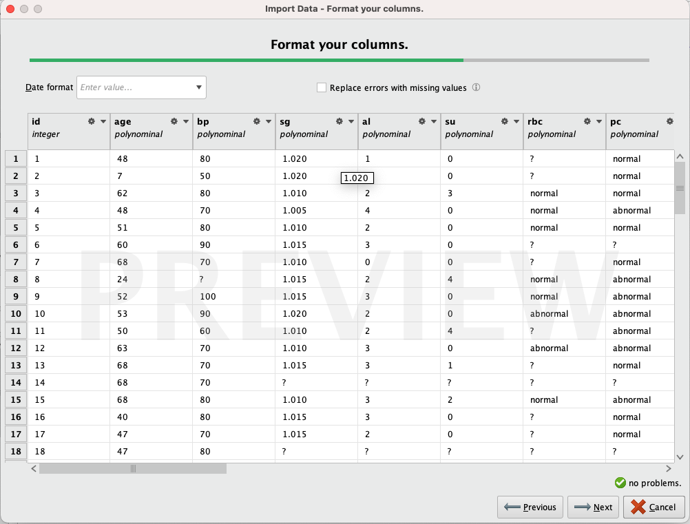
We observe that most of the attributes are recognized as 'polynomial,' even though only a few of them should be. We edit all the attributes, assigning the types defined in the table above. Remove rows that might cause issues (for example, if a row contains 'no' in the 'class' column. It could be interpreted as 'notckd,' but since it's a single value and we are not certain, removing it won't cause problems). Finally, we renamed the attributes to make their names more descriptive and easier to work with.
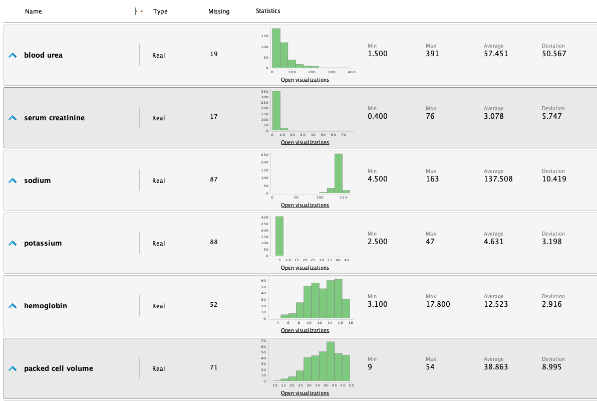
Statistics
Once the data is loaded into RM, we can study the following statistics:
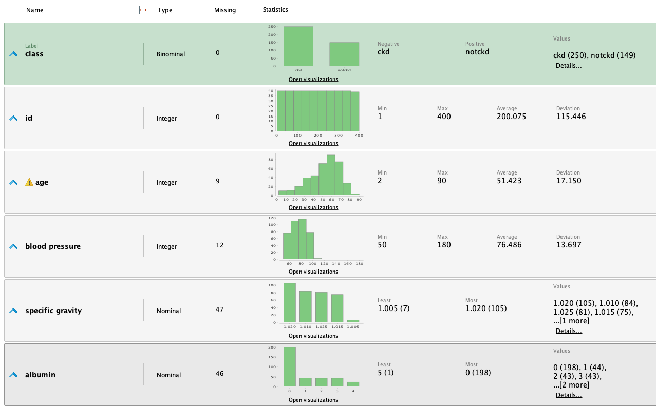
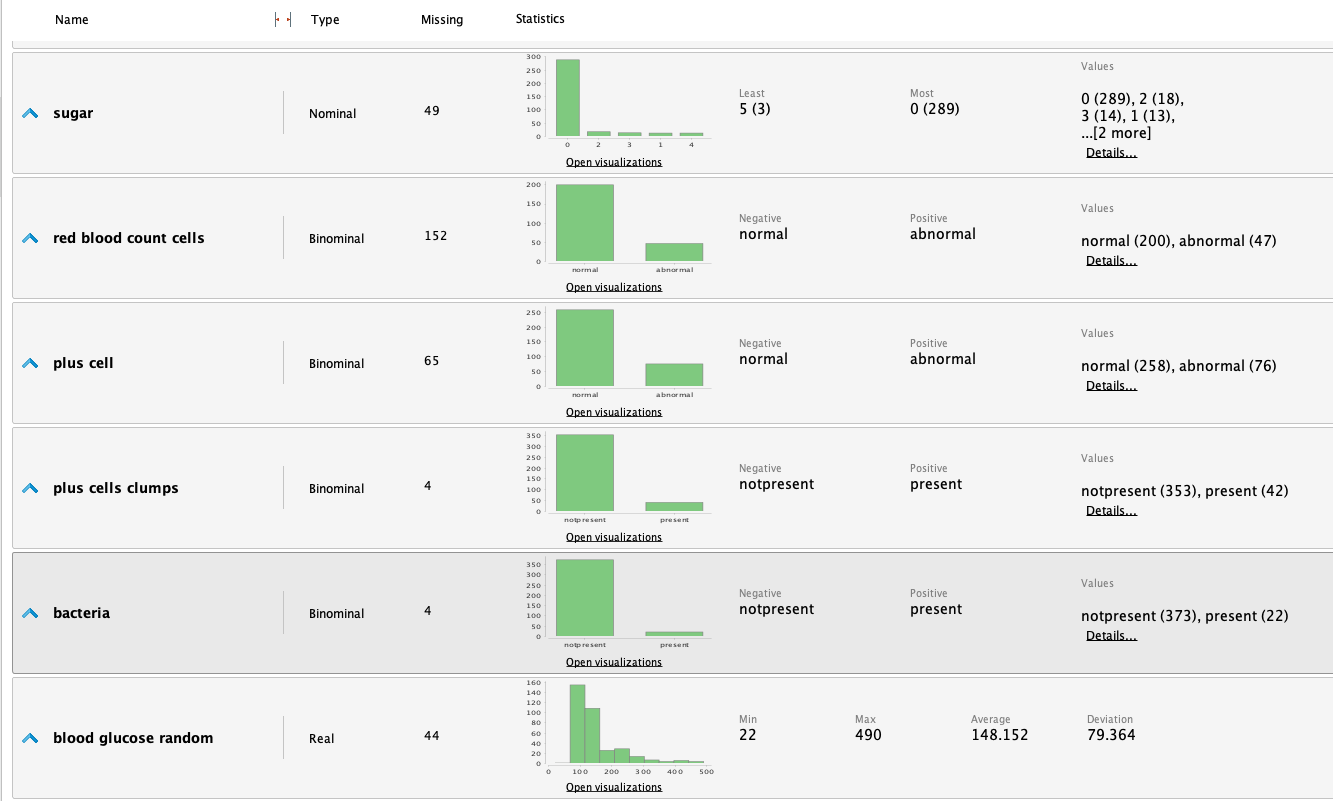
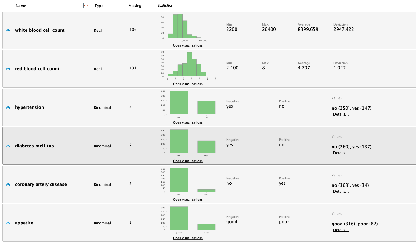
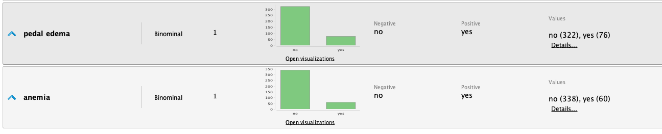
From the statistics, we highlight the following observations:
- It's a dataset with many missing values for various attributes.
- The 'class' attribute is fairly balanced.
-
The 'potassium' column contains 2 outliers: we assume that a
decimal point was omitted in the input, as the values 47 and
39 would make more sense if they were 4.7 and 3.9.
- We edit these datapoints in the dataset and rerun the statistics.
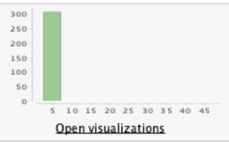
Before
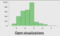
After
-
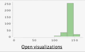
The 'sodium' column contains another outlier of value 4,5
(values range between 100 - 163)
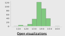
- Since there are many missing values (87) for this column, we just delete this value, and running the statistics again we can see the next improvements:
Before
After
-
We see in the initial statistics that some attributes are
heavily unbalanced. This can be improved using logarithmic or
exponential funcions to balance the data an improve results.
- Blood pressure
- Albumin
- Sugar
- Blood glucose random
- Blood urea
- We have observed that the Serum creatinine levels appear to be significantly unbalanced. Upon closer examination of the data, we have identified values such as 76, 32, and 24 mg/dl, which are considerably elevated for a typical individual. A brief research indicates that normal values typically range from 0.7 to 1.3 mg/dl, significantly lower than the values that have raised suspicion. Nonetheless, it's important to consider that these values could be attributed to an unwell patient, making them potentially valid. As a result, we have decided to retain these values in their current form. However, we will remain vigilant regarding their potential impact in the future and conduct a more thorough investigation to determine whether they should be classified as outliers.
Dealing with missing values
When examining the statistics, we notice a substantial presence of missing values. Dealing with this issue offers several approaches. We can choose to substitute them with averages or logically derived data, remove rows containing missing values entirely, or employ machine learning methods to predict the missing values based on available data.
Nevertheless, it's essential to be cautious with these techniques, as they might introduce inaccurate data into the system, potentially compromising or deteriorating the final outcome. Additionally, some algorithms are capable of accommodating missing values. Therefore, in our initial version, we will work with the missing values in their current state. If we identify room for improvement, we can explore these techniques at a later stage.
Studying correlated attributes
Once in RapidMiner we can quicly make use of the Correlation matrix operator to find out more info about these attributes
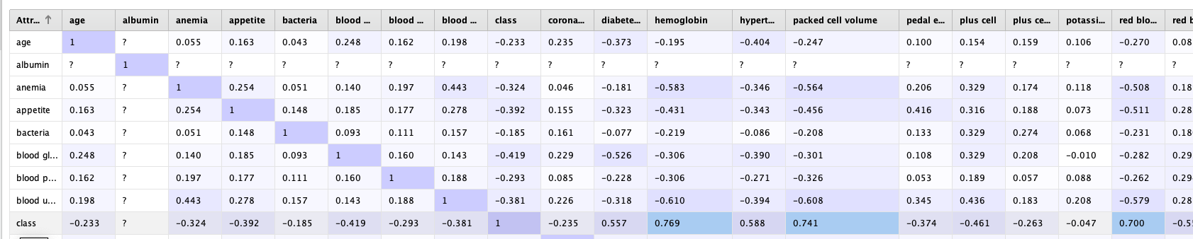
At first sight we cant find heavily correlated attributes. The most correlation is between the class atribute with Hemoglobin, packed cell volume and red blood count. However the correlation value does not exceed 0.77, so for now we will leave it as it is.
Modelling
Now to the fun part! We will start processing the data with some ML models to find out if we can predict the target value. Since we are going to try to classify new incoming data into two possible outcomes ckd and notckd, we can clearly identify this as a classification problem, therefore we will make use of classification models.
Some classification models that we can make ous of are Logistic regression, Linear discriminant analysis, KNN and Naive bayes
Validation
To assess the performance of the models, we will employ the Cross-Validation operator from RM, using a 5-fold strategy. Cross-validation involves dividing the dataset into five subsets, and the model is trained and validated five times. Each fold serves as the validation set exactly once, ensuring thorough assessment. This approach not only utilizes all available data but also tests the model's ability to generalize to unseen data, making it a robust validation method.
Feature selection
We can see that there are many attributes with information here. Some of these attributes may not be useful, and may also impact negatively not only the performance in terms of efficiency, but the outcome itself.
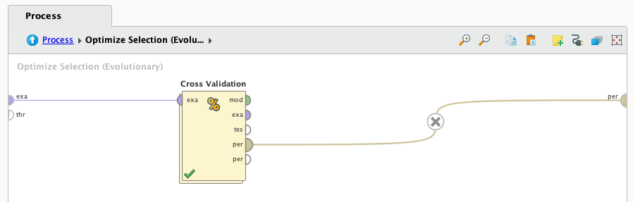
To analyze these attributes in search of the most useful ones, we can employ various techniques. However, we will opt for the RM operator called Optimize Selection (evolutionary). This operator essentially repeats the entire process multiple times, selecting different attributes each time and evaluating their performance. Ultimately, this operator will help us identify the most useful attributes, resulting in improved performance. On a side note, we choose 'evolutionary' because it is the option most likely to prevent reaching a local maximum.
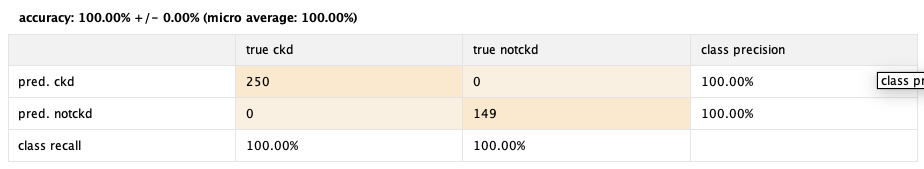
Logistic regression
Lets work with the first algorithm, logistic regression. We plug it in the cross validation operator and press play
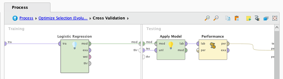
After it finishes processing we look at the results:
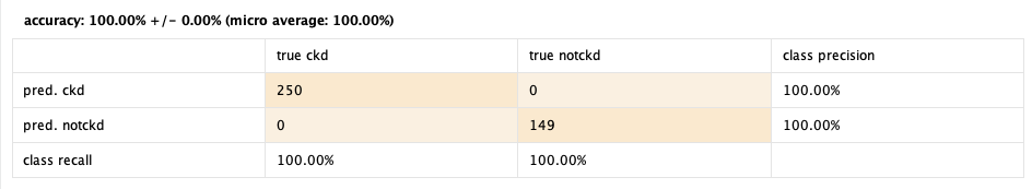
100%! 🤯
Seems a little too good to be true, doesn't it? There may be some issues with the data that leads to such a good, but false outcome. Also, playing around with the operators we observed that the Optimize Selection operator raised the performance from 98% to 100%. Even tough this may be a misleading result, we will keep working with the other models to see how they perform.
Linear discriminant analysis
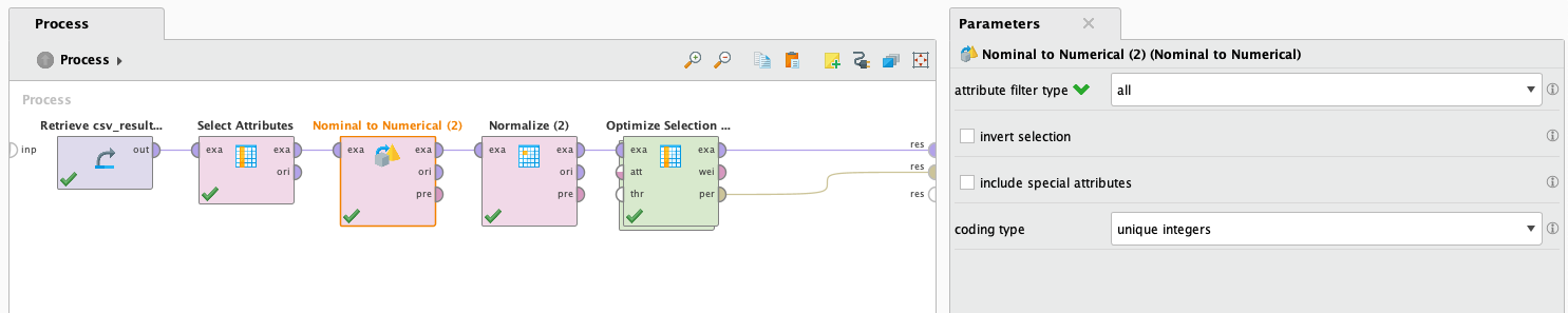
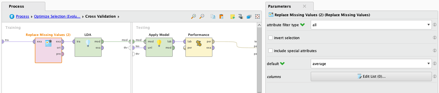
LDA does not support working with missing values, but we are going to try it anyways filling the data with average values. This is not a good idea because its made up information, but we are going to try it anyways just to see how it performs. Also, it doesn't support binomial or polynomial attributes. To solve this we will use the operator Nominal to numerical, which will transform the values of binomial and polynomial attributes to numerical ones.
After it finishes processing we look at the results:
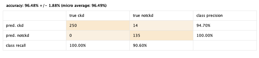
96.48% 😎
Not bad to have so many made up values. playing around with the operators we found out that when leaving out the rows with missing values (a lot of rows), it had a 61% success performance, and autocompleting missing values upgraded it to 90%. This is probably due to the very little examples in the dataset that have all the attributes complete. Also we noted that the operator Optimize Selection raised the performance from 90% to 96%! We can clearly see that this operator rocks.
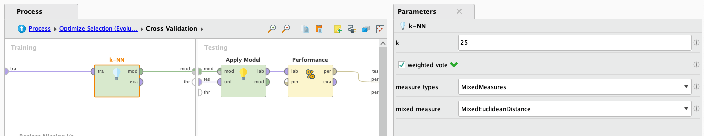
KNN
KNN or k-nearest neighbours is a computationally expensive algorithm, but since we wont be working with a huge dataset we will try it out and see how it performs.
After it finishes processing we look at the results:
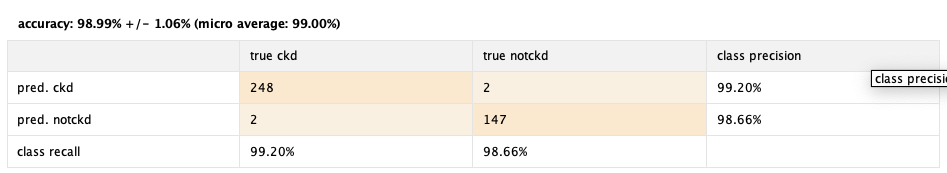
98.99% 😱
Really good performance! We accomplished this after some tweaking with the knn operator parameters, and also some data preprocessing. Running it in the first instance resulted in 61% performance. After that we implemented the Normalize operator, which normalized every attribute. This is especially good for KNN, upgrading it's peformance to 91%. After this we tweaked the k parameter of the KNN operator, finding out that the values around "25" turned out to be the most performant ones, upgrading the performance to 95.49%. Lastly, we used the trusty operator Optimize Selection, reaching the showed result, almost 99%🚀.
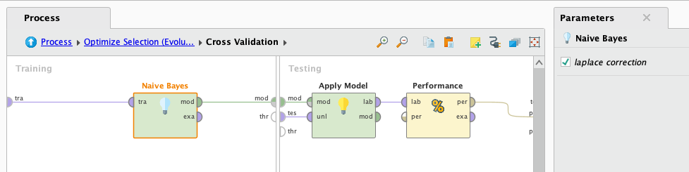
Naive Bayes
This algorithm assumes independence of features and may not work well with highly correlated features. However as we saw previously there are no higly correlated attributes, so we are going to give it a chance and see how it performs:
After it finishes processing we look at the results:
100% 🤑
Again, amazing performance. And the operator Optimize Selection, did it's thing again, turning an already optimal 99% efficiency to a 100%.
Conclusions
All these performances seem too good to be true, and this is a bit unsetteling. However after some time thinking of reasons it may work too good, I couldn't find a satisfactory explanation other than: It really works!
After all, thanks to the cross validation operator, the models should not be suffering of overfitting, which should be a reason to have such high performance. To continue working on this, the best approach to further validate the models would be to use another dataset that is very similar and already classified, and test the performances to see if it actually works as well as it shows.
Lastly, the MVP of this study case will be the operator Optimize Selection, wich optimized every model, from a resource efficiency point of view, to the overall performance of all of them. 🥳